Electronic Configuration of Atoms | Chemistry Class 11 - NEET PDF Download

What is Electronic Configuration?
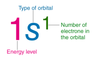
- The distribution of electrons of an atom in its various shells, subshells, and orbitals is known as electronic configuration.
- Electronic configurations of atoms follow a standard notation in which all electron-containing atomic subshells (with the number of electrons they hold written in superscript) are placed in a sequence.
 Example of Electronic Configuration
- For example, the electronic configuration of sodium is 1s22s22p63s1.
- Valence shell or outermost shell → nth shell
- Penultimate shell-Inner to outermost shell → (n -1) shell
- Anti Penultimate shell → (n - 2) shell
Electronic configuration can be expressed in the following ways :
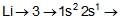
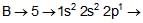
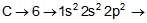
(i) Orbital notation method: nlx
Li → 3 → 1s2 2s1
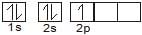
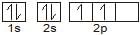
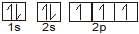
(ii) Orbital diagram method :
Li → 3 → 
(iii) Condensed form :


Electronic Configuration of ions :
To write the electronic configuration of ions, first, write the electronic configuration of the neutral atom and then add (for a negative charge) or remove (for a positive charge) electrons in the outer shell according to the nature and magnitude of charge present on the ion. e.g.
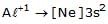
Al → [Ne]3s2 3p1,
 ,
,

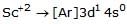
Similarly, in the case of transition elements, electrons are removed from the nth shell e.g. 4th shell in the case of 3 d series.
Cl : [Ne] 3s2.3p5
Cl- : [Ne] 3s2.3p6
Exceptional configuration of Copper and Chromium
Expected configuration Cr - 24 -> [Ar] 4s2 3d4
Observed configuration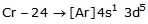
Expected configuration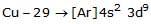
Observed configuration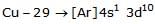
The above exceptional configuration can be explained based on the following factors.
Symmetrical Electronic Configuration
It is a well-known fact that symmetry leads to stability, orbitals of a subshell having a half-filled or full-filled configuration (i.e. symmetrical distribution of electrons) are relatively more stable. This effect is dominating in the d and f subshells.
d5, d10, f7, f14 configurations are relatively more stable.
Exchange Energy
It is assumed that electrons in degenerate orbitals, do not remain confined to a particular orbital rather they keep on exchanging their positions with electrons having the same spin and the same energy (electrons present in orbitals having the same energy). Energy is released in this process known as exchange energy which imparts stability to the atom. The more the number of exchanges, the more will be energy released, and more the energy released stability will be.
You may note that the exchange energy is at the basis of Hund’s rule that electrons which enter orbitals of equal energy have parallel spins as far as possible. In other words, the extra stability of half-filled and completely filled subshell is due to:
(i) relatively small shielding,
(ii) smaller coulombic repulsion energy, and (iii) larger exchange energy.
Magnetic moment (m):
It is the measure of the magnetic nature of a substance
where n is no. of unpaired electrons.
When m = 0, then there is no unpaired electron in the species and it is known as a diamagnetic species.
These species are repelled by magnetic fields.
When  , for paramagnetic species. These species have unpaired electrons and are weakly attracted by the magnetic field.
The formula for the magnetic moment is:
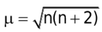
where n= no. of unpaired e-
Ques. Calculate the magnetic moment of these species
(i) Cr
Solution:
(i) Cr: No. of unpaired electrons = 6.
= 
 BM.
BM.
Generally, species having unpaired electrons are coloured or impart colour to the flame. Species having unpaired electrons can be easily excited by the wavelengths corresponding to visible lights and hence they emit radiations having characteristic colour.
|
114 videos|263 docs|74 tests
|
FAQs on Electronic Configuration of Atoms - Chemistry Class 11 - NEET
| 1. What is an electron configuration? |  |
| 2. How is the magnetic moment (m) related to electron configurations? | |
| 3. What is the radial wave function (R) in electron configurations? | |
| 4. How does the radial probability density (R2) relate to electron configurations? | |
| 5. What is the significance of the angular wave function (QF) in electron configurations? | |


Previous Year Questions with Solutions
,Semester Notes
,Summary
,shortcuts and tricks
,Electronic Configuration of Atoms | Chemistry Class 11 - NEET
,study material
,Objective type Questions
,ppt
,MCQs
,Extra Questions
,mock tests for examination
,Electronic Configuration of Atoms | Chemistry Class 11 - NEET
,Viva Questions
,practice quizzes
,Important questions
,Electronic Configuration of Atoms | Chemistry Class 11 - NEET
,Free
,video lectures
,past year papers
,Sample Paper
,Exam
;


Electronic Configuration of Atoms Free PDF Download
Importance of Electronic Configuration of Atoms
Electronic Configuration of Atoms Notes
Electronic Configuration of Atoms NEET Questions
Study Electronic Configuration of Atoms on the App
|
© EduRev
|
Education Revolution
|


|


