Efficiency Of Single Phase Transformers | Electrical Machines - Electrical Engineering (EE) PDF Download

Efficiency of Single Phase Transformers
(Refer Slide Time: 01:04)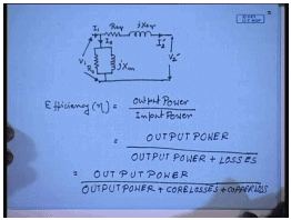
In the last lecture, we have seen how to obtain the parameters of the approximate equivalent circuit of the single phase transformer; the approximate equivalent circuit looks like this. This is the supply voltage V 1 magnetizing current I 0, supply current I 1, R e q, j X e q is the referred load current I 2 dash, and this is the referred load voltage V 2 dash. While this equivalent circuit is important for finding out different performance parameters from a user point of view certain performance parameters are very important. For example, one of the most important performance parameter is the efficiency of transformer. Now efficiency as in the case of any other power processing equipment for a transformer the efficiency is defined as the symbol is nu is defined as output power divided by the input power.
Now what is the difference between output power and input power? It is the losses. So, this can also be written as output power divided by output power plus losses. Now what are the different losses that can occur in a single phase transformer? We have seen the first element is the core loss resistance. This is the loss due to hysteresis and ac current, and in the equivalent circuit we represent it by a resistance. And the second major loss that can occur is in the winding resistances R e q; therefore, the losses can be broken down into two parts plus core losses plus losses in the winding resistance, this is called the copper loss.
Now even from the equivalent circuit also from the physical principle due to which this losses takes place we can argue that this core loss depend on the applied voltage and frequency. But single phase transformers are normally connected to voltage sources of constant magnitude and frequency; therefore, the core loss occurring in a single phase transformer is more or less constant. It does not depend on the load; however, the losses that are occurring in the winding resistance they do depend on the load current magnitude and it given by I square Req.
(Refer Slide Time: 05:37)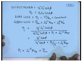
Therefore, in terms of equations we can write output power is equal to V 2 dash I 2 dash cos phi where phi is the load power factor angle. This is same as V 2 I 2 cos phi. Core loss is given by V 1 square by R 0; we indicate it as P core or P iron, and this is usually constant. Copper loss diluted as P Cu equal to I 2 dash square R e q or this I 2 square R e q dash same thing I 2 square R e q dash. Therefore, efficiency nu can be written as which again can be written as. In a general transformer the variation of V 2 dashed with I 2 dashed is usually very small.
So, for all practical purpose V 2 dash can be assumed to be to remain constant at its rated value. Further more if we assume that the load power factor also is constant, then we can say that the efficiency depends only on the magnitude of the current I 2 dash. And it will be interesting to find out at what value of I 2 dash this efficiency becomes maximum? Now if you look at the expression of the efficiency we see that this V 2 dashed cos phi divided by V 2 dashed cos phi plus P i by I 2 dash plus I 2 dash R e q of which the numerator is constant, the first term of the denominator is constant; only these two terms are functions of I 2 dash.
For nu to be maximum the denominator should be minimum. Now up the denominator the first term is constant. So, the sum of the second and third term should be minimum. So, differentiating this quantity with respect to I 2 dash we get the condition for maximum nu max is P i equal to I 2 dash square R e q; that is P i equal to P cu. The load current at which the fixed iron loss becomes equal to the core loss is the load current at which the efficiency of a single phase transformer is maximum. Now while the load parameters are given it is possible to find out I 2 dash and the efficiency under any given load condition. It is the practice usually is to find out these values from the test data. The other day we have seen how to find this loss component.
We have seen that in the open circuit test; we connect a wattmeter. The wattmeter reading is equal to the core loss, because there is no current almost no current flowing in the transformer. The no load current is very small. Similarly, on the short circuit test data we argued that the magnetizing current is very small; therefore, the core loss is very small. So, the wattmeter reading actually represented the copper loss. Now short circuit test is usually done at the rated current; therefore, the value we get is the full load copper loss from short circuit test. Similarly from the open circuit test we get the iron loss which is independent of the load current and constant.
(Refer Slide Time: 12:02)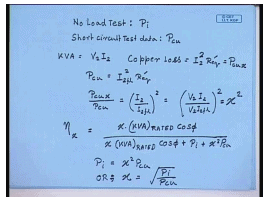
So, let us say from the no load test data we get the wattmeter reading to be P I; short circuit test data we get the reading to be P cu. Then from this data we can find out the load at which the transformer efficiency will be maximum. The load the KVA load on a transformer is equal to V 2 I 2 at any load current I 2; the corresponding copper loss equal to I 2 square R e q dash. The full load copper loss as obtained for circuit test P cu, let us say this is at x fraction of load; P cu at full load is equal to I 2 full load square R e q dash. So, P cu x by P cu equal to I 2 divided by I 2 full load square. This is same as V 2 I 2 divided by V 2 I 2 full load square which is same as the fractional load x square.
Therefore, the efficiency at any fractional load x can be written as efficiency at a fractional load x equal to x times the KVA rating of the transformer into cos phi divided by x times rated KVA to cos phi plus P i plus x square P cu where P cu is the full load copper loss of the transformer. And we have seen that the fractional load at which the efficiency will be maximum then P i is equal to x square P cu or x equal to square root P i by P cu. So, this is the fractional load at which the transformer efficiency will be maximum. Now this realization has something to do with the design of a transformer. It is natural that we would like the transformer to be as efficient as possible, because that will reduce the energy loss which means that transformer should ideally be always operating at the load at which its efficiency is maximum.
However, it is not possible to guarantee that for all types of transformers; for example, the transformers that are used in transmission are almost always loaded up to their full capacity. Therefore, while designing a transmission transformer we like to make sure that its maximum efficiency occurs near the rated load; however, the situation is very different for distribution transformer. Distribution transformer for a large part of the day remains lightly loaded or even remains on no load. Therefore for a distribution transformer it is important to design the transformers such that the maximum efficiency does not occur at full load but at a reduced load.
Usually for a distribution transformer it is not unusual to have the loading corresponding to the maximum efficiency at around 60 to 65e percent. From this discussion we also can conclude one more thing that getting the transformer efficiency at a particular load does not give the full picture, because the loading of a transformer can vary over a day. Normally it is expected that the loading pattern of a transformer will repeat over every day in a season at least.
(Refer Slide Time: 18:51)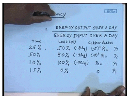
Therefore more useful parameter in order to find out the performance of a transformer is called the all day efficiency; how do I define all day efficiency? This is defined as energy output of the transformer over a day divided by energy input to the transformer over the day. Now had the transformer been uniformly loaded over the day then this all day efficiency would have been same as the efficiency of the transformer at a given load; however, it is not so. Let us say the transformer is loaded, say 25 percent of the time at let us say 50 percent of the load time load that is x. Then 50 percent of the time let us say is loaded at 80 percent, and let us say 10 percent of the time it is loaded at 100 percent, and for the rest of the 15 percent of the time it remains at no load.
Now if this transformer has a copper loss of P cu at full load, and P i is the core loss, then the losses will be copper losses particularly will be 0.5 square P cu, here it will be 0.8 square P cu, and here it will be P cu, and here it will be 0. The core loses, however, will always be P i, P i, P i, here also P i. Let us further assume that these loads have power factor let us say at 50 percent, let us say this power factor is 0.8 lagging, this power factor is 0.9 lagging, this power factor is 0.95 lagging, and here since there is no current we do not mention the load power factor. So, let us calculate, what will be the all day efficiency?
(Refer Slide Time: 23:02)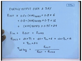
The energy output over a day let us say the transformer KVA rating is KVA rated then the energy output over a day is equal to 50 percent 0.5 into 25 percent of a day that is 6 hours one-forth is 6 hours which remains loaded at 50 percent. So, 0.5 into KVA rated into power factor is 0.8 into 6 hours, so many kilowatt hour at 25 percent of the loading plus 85 percent of the loading into KVA rated into power factor it is 0.9 into 12 hours plus 100 percent of the loading that is 1 or KVA rated into 0.95 is the power factor into 10 percent of the time that is 2.4 hours plus 0 percent loading that is no output for another 3.6 hours.
So, this is the total energy output of the transformer. What is the total energy input? E in equal to E out plus E loss; how do I calculate the losses? Losses we can find since we know that the core loss remain constant at any loading, and the copper loss is given by these values. So, total energy loss is equal to E loss equal to 24 hours into P i plus 6 hours at 50 percent of the load. So, 0.25 into P c u into 6 hours plus 50 percent of the time at 80 percent of the load; so 0.64 into P cu into 12 hours plus rate in full load for 10 percent of the time that is P c u into 2.4 hours. So, this is the total energy loss. So, nu all day equal to E out divided by E out plus E loss. This is how one should calculate the all day efficiency of a single phase transformer.
And that the only data we need to calculate this all day efficiency are the copper loss at full load which can be obtained from short circuit test data and the core loss which can be obtained from open circuit data and of course, the loading pattern of the transformer. If this data are given then the all day efficiency of a transformer can be found. Now one of the effect of this loses is to generate heat and increase the temperature of the transformer. We have found out how from open circuit and short circuit test we can find out the core loss and the copper loss of a transformer; however, during open circuit test there is no root current going. So, the transformer is subjected to only core loss. Similarly in the short circuit test the core loss is negligible; the transformer is subjected to only copper loss.
So, in none of this tests this transformer usually sees both the loss occurring simultaneously; therefore, it is not possible to find out experimentally the temperature rise that will occur in a transformer when it is actually used. However, this test is very important from user point of view because during use the transformer will be supplying load. Hence it will be subjected to core loss and copper loss simultaneously, and as a result the final statistic temperature rise will be determined by the total loss. Now it is possible to find out the temperature rise of a single phase transformer by test but not from no load test or a short circuit test. The test by which we can find out the temperature rise of a single phase transformer is called the back to back test or Sumpner’s test.
(Refer Slide Time: 30:17)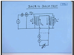
As we will see shortly this test cannot be performed with a single transformer; we need at least two transformers, and these two transformers should preferably be identical at least their voltages should be very close or identical. The way it is done is the two identical transformers are taken. Their primary are connected in parallel, and it is supplied from a related voltage source, Of course, some meters are to be connected means we have to connect an ammeter; we have to also connect a wattmeter. The secondaries of the transformers are connected in series with this polarity. Here again another ammeter is connected, another wattmeter is connected, and these secondary’s are supplied from a variable voltage source.
So, how do you subject the transformers to simultaneous core loss and copper loss just like this. Let us assume that let us apply superposition theory; let us assume one source at a time. So, you replace this by a short circuit. Since these two transformers are identical the voltage generated across the secondary winding will be same provided since they are supplied from the same source; therefore, there will be no circulating current flowing in the secondary’s, because the induced voltage in one will oppose the other. The current drawn by these transformers will be only the no load current of these two transformers. Similarly, if we short the source V 1 and consider the contribution of the source V 2 we see that the current flowing in the secondary windings we will see to short at primary couple to them.
Therefore, the current flowing through the transformer can be controlled by controlling this voltage cells to be the rated current of these two transformers, and the power drawn will be the copper loss of the two transformers. Therefore, when source V 1 is present, V 2 is shorted; the power drawn is simply the core loss of the two transformers. Now V 1 is shorted and V 2 is applied then the power loss power drawn is the copper loss of the two transformers. When both are applied let us say if current is circulated I 2 current circulates this way; therefore, the reflection current here it will be I 2 dash flowing in this direction, and similarly I 2 dash flowing in this direction. However, if these two transformers are identical then this I 2 dashed current will circulate only in the transformer primary winding the current drawn from the source we still be 2I 0.
Therefore during this test the total power drawn from the two sources V 1 and V 2 will be the sum of the core loss and the copper loss and since the transformers will be subjected simultaneously to core loss and copper loss their temperature rise will be same as that when they will be in actual use. So, in this case we see that we can simulate actual loading of the transformers without drawing the required power from the source; that is why it is called a back to back test, and this is a general principle. In many electrical machines we will see such equivalent circuits for back to back tests, because it is important for any electrical equipment to be tested at its rated capacity.
However, it is also inconvenient particularly the equipment is of large rating to actually load the equipment and test it. Therefore for almost all electrical machines some form of back to back test becomes important, and this is the way the back to back test is performed on a single phase transformer. We will end this lecture by looking at an exercise of how to find out the equivalent circuit parameters of a single phase transformer from test data and how to find the efficiency.
(Refer Slide Time: 37:15)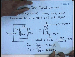
Let us say we have 200 volts by 400 volt transformer single phase transformer; KVA rating is 4 KVA. Let us say the no load test data of this transformer is the voltage rating is no load test is of course done on the LV side. The test data is voltage reading is 200 volt since rated voltage is to be applied; the current drawn is 0.7 ampere, and the wattmeter reading is 35 watts. The short circuit test data this is done on the HV side; the applied voltage is 30 volts. The circulating current is 10 ampere, and the wattmeter reading is 90 watts. How do I find out the equivalent circuit parameters of this transformer? Then at no load the approximate equivalent circuit of the transformer looks like this.
This voltage applied is 200 volts. This is j X m, this is R 0, this is the no load current I 0, this is the magnetization current I m, and this is the core loss current I c. The phasor relationship is. So, if this is the applied voltage V LV then I m will lag V LV by 90 degree, and I c will be in phase will be in; therefore, the total no load current I 0 will be at a power factor angle phi 0 respect to the applied voltage. Now from the no load test data these voltage is given to be 200 volt, and the no load current I 0 equal to 0.7 amperes. Therefore, the no load power factor cos phi 0 equal to the V LV I 0 W 0 divided by V LV 0; this is equal to 35 divided by 200 into 0.7. Let us say 0.25, but what is I m? I m equal to V LV by X m, but this is also equal to I 0 sin phi 0, and I c equal to V LV by R 0 equal to I 0 cos phi 0.
(Refer Slide Time: 42:33)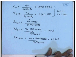
From the given data therefore, X m equal to V LV divided by I 0 sin phi 0. This comes as 200 and 95.08 ohm, and R 0 equal to V LV by I 0 cos phi 0. This comes to 1.143 kilo ohms. It should be remembered that both that both these values are referred to LV side, since that is where the test was performed. As we have seen that there are some advantages in expressing them in per unit; for that we will have to find out what is Z base on the LV side. So, Z base equal to V LV rated square divided by rated KVA of the transformer. Hence R 0 p. u equal to R 0 into rated KVA of the transformer divided by V LV rated voltage square. This comes to 114.3. Similarly by the same formula X m p. u equal to X m into KVA base rated KVA divided by; this comes to 29.508. So, we have seen how to find out the shunt parameter branches of the equivalent circuit and express them in per unit. Let us now shift our attention to the series parameters.
(Refer Slide Time: 45:56)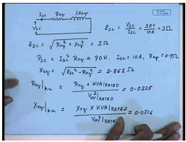
In the short circuit test we can neglect the shunt branch the equivalent circuit is somewhat like this. The applied voltage is V sc, the current is I sc, this resistance is R e q, this is j X e q. Hence Z sc that is mod Z sc equal to V sc by I sc; from the given data this is 30 volts by 10 amperes equal to 3 ohms. Therefore, Z sc equal to square root R e q square plus X e q square equal to 3 ohm. Similarly the power P sc short circuit power equal to I sc square R e q; this is given to be 90 watts. I sc equal to 10 ampere; hence, R e q equal to 0.9 ohm, X e q then will be Z sc square minus R e q square; this comes to 2.862 ohms.
Now both the values of R e q and X e q are found referred to the HV side, since short circuit test is done on the HV side; again this can also be converted to per unit. So, R e q per unit will be equal to R e q into rated KVA of the transformer divided by now HV side rated voltage square. This comes to 0.0225 and X e q per unit will be equal to X e q into KVA rated divided by V HV square rated. This will give you 0.0716.
(Refer Slide Time: 49:05)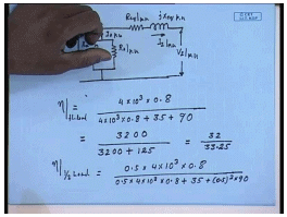
Therefore, the complete equivalent circuit is per unit of this transformer will be. This is X n P u, this is R 0 P u, this is R e q P u; this is j X e q P u. Here you will get V 2 in per unit, here you get I 2 in per unit, here you will get I 1 in per unit, this is I 0 in per unit. So, this is how you get the equivalent circuit parameters of a single phase transformer from short circuit and open circuit test data. Now if I want to find out for the same transformer what will be the efficiency, let us say at 50 percent of the load? First let us find out what will be the efficiency at 100 percent of the load? At 100 percent of the transformer KVA rating is 4 KVA. So, at 100 percent of the load, and let us say at 0.8 power factor the output power is 4 into 10 to the power 3 watts into power factor is 0.8 divided by the output power is 4 into 10 to the power 3 into 0.8 plus the copper loss; the core loss is 35 watts plus 100 percent; that is at full load the copper loss is 90 watts.
So, at full load the efficiency is 3200 divided by 3200 plus 125, 32 divided by 33.25. This will be the full load efficiency nu full load. If I reduce it to half load then nu half load will be, at half load the power output will be 0.5 and at the same power factor 4 into 10 to the power 3 into 0.8 divided by 0.5 into 4 into 10 to the power 3 into 0.8 plus 35 plus 0.5 square into 90. This will be the efficiency at half load. It will be interesting to find out at what load the efficiency of the transformer will be maximum; let that load be X.
(Refer Slide Time: 52:57)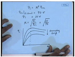
Then we know from the condition of maximum efficiency at the loading at which efficiency is maximum; there p i equal to x square P cu where x is the fractional load. From the short circuit test data P cu at full load equal to 90 watts, and P i equal to 35 watts. So, at what load the efficiency will be maximum? The maximum efficiency will occur at x equal to P i by P cu square root; this is equal to 35 by 90 square root. So, at this load the efficiency will be maximum. It is to be noted that although the actual value of this efficiency is dependent on the power factor the load at which efficiency over the maximum efficiency occurs is independent of the power factor. So, the plot of efficiency versus percentage load will look somewhat like this, at 0 it is 0, but at a different power factor the efficiency curves will pick at the same point. So, these are for decreasing cos phi.
|
19 videos|124 docs|25 tests
|
FAQs on Efficiency Of Single Phase Transformers - Electrical Machines - Electrical Engineering (EE)
| 1. What is the efficiency of a single-phase transformer? |  |
| 2. How is the efficiency of a single-phase transformer affected by the load? | |
| 3. What are the main factors influencing the efficiency of a single-phase transformer? | |
| 4. How can the efficiency of a single-phase transformer be improved? | |
| 5. Is there a minimum efficiency requirement for single-phase transformers? | |


Extra Questions
,Exam
,Sample Paper
,video lectures
,Efficiency Of Single Phase Transformers | Electrical Machines - Electrical Engineering (EE)
,mock tests for examination
,Efficiency Of Single Phase Transformers | Electrical Machines - Electrical Engineering (EE)
,MCQs
,Summary
,Objective type Questions
,Viva Questions
,Semester Notes
,practice quizzes
,Previous Year Questions with Solutions
,Important questions
,ppt
,study material
,Efficiency Of Single Phase Transformers | Electrical Machines - Electrical Engineering (EE)
,past year papers
,Free
,shortcuts and tricks
;


Efficiency Of Single Phase Transformers Free PDF Download
Importance of Efficiency Of Single Phase Transformers
Efficiency Of Single Phase Transformers Notes
Efficiency Of Single Phase Transformers Electrical Engineering (EE) Questions
Study Efficiency Of Single Phase Transformers on the App
|
© EduRev
|
Education Revolution
|


|


