


All Exams >
Class 6 >
How to become an Expert of MS Excel >
All Questions
All questions of Excel Tips for Class 6 Exam
Microsoft Excel is a powerful ________- a)Word processing package
- b)Spreadsheet package
- c)Communication S/W Package
- d)DBMS package
Correct answer is option 'B'. Can you explain this answer?
Microsoft Excel is a powerful ________
a)
Word processing package
b)
Spreadsheet package
c)
Communication S/W Package
d)
DBMS package
|
|
Utkarsh Joshi answered |
Microsoft Excel is Microsoft's general-purpose spreadsheet program for Windows, used for data analysis and display. It is commonly used in a business environment since it is part of the Microsoft Office package. Microsoft Excel is an extremely powerful tool, which is used by millions of people everyday. Functions tailored to a specific task can be programmed into Excel to extend its capabilities with customised analysis tools.

You can move a sheet from one workbook into new book by- a)From Edit menu choose Move or Copy sheet, mark the Create a ccopy and Click OK
- b)From Edit menu choose Move of Copy then choose (Move to end) and click OK
- c)From Edit menu choose Move or Copy then select (new book) from To Book list and click OK
- d)None of above
Correct answer is option 'C'. Can you explain this answer?
You can move a sheet from one workbook into new book by
a)
From Edit menu choose Move or Copy sheet, mark the Create a ccopy and Click OK
b)
From Edit menu choose Move of Copy then choose (Move to end) and click OK
c)
From Edit menu choose Move or Copy then select (new book) from To Book list and click OK
d)
None of above
|
|
Utkarsh Joshi answered |
From Edit menu choose Move or Copy then select (new book) from To Book list and click OK
MS Excel provides the default value for step in Fill Series dialog box- a)0
- b)1
- c)5
- d)10
Correct answer is option 'B'. Can you explain this answer?
MS Excel provides the default value for step in Fill Series dialog box
a)
0
b)
1
c)
5
d)
10
|
|
Anisha Iyer answered |
Explanation:
In MS Excel, the Fill Series dialog box allows users to automatically fill a series of cells with values that follow a specific pattern. When using the Fill Series dialog box, the "Step Value" option allows users to specify the difference between each value in the series.
The default value for the "Step" in the Fill Series dialog box is 1, which means that the series will increase or decrease by 1 for each subsequent cell.
Here's an explanation of each option:
- Option a) 0: This option does not make sense as a step value since it would result in a static series with no change in value.
- Option b) 1: This is the correct answer. The default step value in MS Excel's Fill Series dialog box is 1. This means that if a user fills a series starting from a specific value, each subsequent cell will contain a value that is incremented or decremented by 1.
- Option c) 5: This option is not the default step value in MS Excel's Fill Series dialog box. However, users can manually set the step value to 5 if they want the series to increase or decrease by 5 for each subsequent cell.
- Option d) 10: This option is also not the default step value in MS Excel's Fill Series dialog box. Users can manually set the step value to 10 if they want the series to increase or decrease by 10 for each subsequent cell.
Therefore, the correct answer is option b) 1, as it represents the default step value in MS Excel's Fill Series dialog box.
An Excel Workbook is a collection of ________- a)Workbooks
- b)Worksheets
- c)Charts
- d)Worksheets and Charts
Correct answer is option 'D'. Can you explain this answer?
An Excel Workbook is a collection of ________
a)
Workbooks
b)
Worksheets
c)
Charts
d)
Worksheets and Charts
|
|
Utkarsh Joshi answered |
A workbook is a collection of one or more spreadsheets and charts in a single file.
Concatenation of text can be done using- a)Apostrophe ( ‘ )
- b)Exclamation ( ! )
- c)Hash ( # )
- d)Ampersand ( & )
Correct answer is option 'D'. Can you explain this answer?
Concatenation of text can be done using
a)
Apostrophe ( ‘ )
b)
Exclamation ( ! )
c)
Hash ( # )
d)
Ampersand ( & )
|
|
Utkarsh Joshi answered |
The ampersand (&) calculation operator allow us join text items without using a function. For example, =A1 & B1 will return the same value as =CONCATENATE(A1,B1). In many cases, using the ampersand operator is quicker and simpler than using CONCATENATE to create strings.
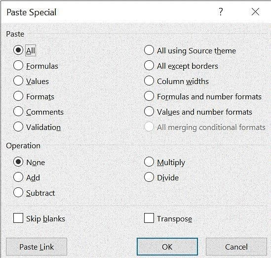
Which of the following you can paste selectively using Paste Special command?- a)Validation
- b)Formats
- c)Formulas
- d)All of above
Correct answer is option 'D'. Can you explain this answer?
Which of the following you can paste selectively using Paste Special command?
a)
Validation
b)
Formats
c)
Formulas
d)
All of above
|
|
Utkarsh Joshi answered |
We can paste formula, value, formats, comments, validation using Paste Special command.
When a row of data is to be converted into columns- a)Copy the cells in row, select the same number of cells in row and paste
- b)Copy the cells in column then choose Paste Special, then click Transpose and OK
- c)Copy the cells then go to Cells then on Alignment tab click Transpose check box and click OK
- d)Select the cells then place the cell pointer on new cell and choose Paste Special, mark Transpose check box and click OK
Correct answer is option 'D'. Can you explain this answer?
When a row of data is to be converted into columns
a)
Copy the cells in row, select the same number of cells in row and paste
b)
Copy the cells in column then choose Paste Special, then click Transpose and OK
c)
Copy the cells then go to Cells then on Alignment tab click Transpose check box and click OK
d)
Select the cells then place the cell pointer on new cell and choose Paste Special, mark Transpose check box and click OK
|
|
Utkarsh Joshi answered |
Transpose (rotate) data from rows to columns or vice versa. To use options from the Paste Special box, click Home > Paste > Paste Special > Transpose
Select the cells then place the cell pointer on new cell and choose Paste Special, mark Transpose check box and click OK
Select the cells then place the cell pointer on new cell and choose Paste Special, mark Transpose check box and click OK
Which elements of a worksheet can be protected from accidental modification?- a)Contents
- b)Objects
- c)Scenarios
- d)All of the above
Correct answer is option 'D'. Can you explain this answer?
Which elements of a worksheet can be protected from accidental modification?
a)
Contents
b)
Objects
c)
Scenarios
d)
All of the above
|
|
Utkarsh Joshi answered |
All elements of a worksheet can be protected from accidental modification.
To protect a worksheet in Excel 2007 and higher versions, click the Review tab, click Protect Worksheet (or Protect Sheet), and click OK.
Excel 2003 and Earlier Versions click Tools > Protection, click Protect Sheet, and click OK.
To protect a worksheet in Excel 2007 and higher versions, click the Review tab, click Protect Worksheet (or Protect Sheet), and click OK.
Excel 2003 and Earlier Versions click Tools > Protection, click Protect Sheet, and click OK.
To select an entire column in MS-EXCEL, press?- a)CTRL + C
- b)CTRL + Arrow key
- c)CTRL + S
- d)None of the above
Correct answer is option 'D'. Can you explain this answer?
To select an entire column in MS-EXCEL, press?
a)
CTRL + C
b)
CTRL + Arrow key
c)
CTRL + S
d)
None of the above
|
|
Bibek Verma answered |
To select an entire column in MS-Excel, you need to follow a specific set of instructions. The correct answer to this question is option 'D' - None of the above. Let's explore the correct method to select an entire column in MS-Excel.
Method to Select an Entire Column in MS-Excel:
Unfortunately, none of the options provided in the question are the correct way to select an entire column in MS-Excel. The following steps describe the correct method:
Step 1: Open the Excel worksheet where you want to select the entire column.
Step 2: Move your cursor to the top of the column you want to select. The column letters are displayed at the top of the worksheet.
Step 3: Click on the letter of the column you want to select. For example, if you want to select column A, click on the letter 'A'. This will highlight the entire column.
Step 4: To select multiple columns, you can hold down the 'Ctrl' key on your keyboard while clicking on the letters of the columns you want to select. For example, to select columns A, B, and C, you would click on the letters 'A', 'B', and 'C' while holding down the 'Ctrl' key.
Step 5: Once the entire column(s) is selected, you can perform various operations on it, such as formatting, entering data, or applying formulas.
Conclusion:
In order to select an entire column in MS-Excel, you need to click on the letter of the column you want to select. Using the 'Ctrl' key allows you to select multiple columns simultaneously. Remember that option 'D' - None of the above is the correct answer in this case.
Ctrl + D shortcut key in Excel will- a)Open the font dialog box
- b)Apply double underline for the active cell
- c)Fill down in the selection
- d)None of above
Correct answer is option 'C'. Can you explain this answer?
Ctrl + D shortcut key in Excel will
a)
Open the font dialog box
b)
Apply double underline for the active cell
c)
Fill down in the selection
d)
None of above
|
|
Jay Goyal answered |
Explanation:
In Excel, the Ctrl + D shortcut key is used to fill down in the selection. This means that it copies the contents and formatting of the cell above the active cell and applies it to the selected cells below. Let's understand this in detail:
Steps to fill down using Ctrl + D:
1. Select the cell or range of cells where you want to apply the fill down operation.
2. Press Ctrl + D on your keyboard.
Example:
Suppose you have a list of names in column A from A1 to A5. You want to copy the name in cell A5 and fill it down to the cells below. Here's how you can use the Ctrl + D shortcut key:
1. Select cell A5.
2. Press Ctrl + D.
Result:
The name in cell A5 will be copied and filled down to the cells below, so now you will have the same name in cells A6, A7, A8, and so on.
Important points to note:
- The Ctrl + D shortcut key only works for filling down. If you want to fill to the right or left, you need to use the Ctrl + R or Ctrl + L shortcut keys, respectively.
- This shortcut key can be used to fill down formulas, values, or any other content in the selected cells.
- It is a quick and efficient way to copy and fill data in a column or a range of cells without the need for manual copying and pasting.
Conclusion:
The Ctrl + D shortcut key in Excel is used to fill down in the selection, copying the contents and formatting of the cell above the active cell and applying it to the selected cells below. It is a handy shortcut for quickly replicating data in a column or range of cells.
Getting data from a cell located in a different sheet is called ________- a)Accessing
- b)Referencing
- c)Updating
- d)Functioning
Correct answer is option 'B'. Can you explain this answer?
Getting data from a cell located in a different sheet is called ________
a)
Accessing
b)
Referencing
c)
Updating
d)
Functioning
|
|
Utkarsh Joshi answered |
Getting data from a cell located in a different sheet is called Cell reference.
There are Three types of Cell reference in Excel
There are Three types of Cell reference in Excel
- Relative
- Absolute
- Mixed
What do you mean by a Workspace?- a)Group of Columns
- b)Group of Worksheets
- c)Group of Rows
- d)Group of Workbooks
Correct answer is option 'D'. Can you explain this answer?
What do you mean by a Workspace?
a)
Group of Columns
b)
Group of Worksheets
c)
Group of Rows
d)
Group of Workbooks
|
|
Mrinalini Khanna answered |
A Workspace refers to a group of Workbooks in Microsoft Excel. A Workbook is a file that contains one or more worksheets, and a Worksheet is a collection of cells where you can enter and manipulate data. Therefore, a Workspace is a collection of multiple workbooks that are opened and displayed together in Excel.
Workbooks
A Workbook is an Excel file that can contain multiple worksheets. It acts as a container for organizing and storing data. Each workbook is independent and can be saved separately. Workbooks can be used to store different types of data or related data that need to be kept separate.
Worksheets
A Worksheet is a single sheet within a workbook. It is made up of a grid of cells where you can enter and manipulate data. Each worksheet has a unique name and can have different formats, formulas, and data. Worksheets are used to organize and analyze data within a workbook.
Workspace
A Workspace is a feature in Excel that allows you to group and manage multiple workbooks together. It provides a way to organize related workbooks and switch between them quickly. When you save a Workspace, Excel remembers the arrangement and location of each workbook, making it easy to reopen the entire group of workbooks later.
Benefits of using Workspace
1. Organization: Workspaces help in organizing related workbooks by grouping them together. This makes it easier to find and access specific workbooks when needed.
2. Efficiency: Instead of opening each workbook individually, you can open a Workspace to simultaneously open multiple workbooks. This saves time and makes it more efficient to work with multiple files.
3. Quick Navigation: Within a Workspace, you can easily switch between different workbooks using the tabs at the bottom. This allows for quick navigation and easy referencing of data.
4. Preserving Layout: When you save a Workspace, Excel saves the arrangement and location of each workbook. This means that when you reopen the Workspace, the workbooks will be opened in the same layout as before, preserving your work progress.
In conclusion, a Workspace in Excel refers to a group of Workbooks that are opened and displayed together. It helps in organizing, managing, and quickly accessing multiple workbooks, providing a more efficient way to work with data.
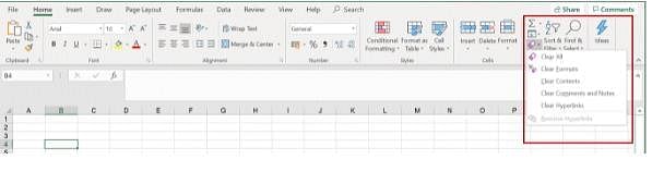
If you need to remove only the formatting done in a range (numbers and formula typed there should not be removed), you must- a)From Edit menu choose Clear and then Formats
- b)From Edit menu choose Delete
- c)Click on Remove Formatting tool on Standard Toolbar
- d)Double click the Format Painter and then press Esc key in keyboard
Correct answer is option 'A'. Can you explain this answer?
If you need to remove only the formatting done in a range (numbers and formula typed there should not be removed), you must
a)
From Edit menu choose Clear and then Formats
b)
From Edit menu choose Delete
c)
Click on Remove Formatting tool on Standard Toolbar
d)
Double click the Format Painter and then press Esc key in keyboard
|
|
Anirban Saini answered |
Explanation:
Removing formatting in a range means clearing only the visual appearance of the cells without affecting the data or formulas within them. Here's how you can do it:
Steps to Remove Formatting in a Range:
1. From Edit Menu:
- Click on the "Edit" menu at the top of the Excel window.
- Choose the "Clear" option from the dropdown menu.
- Select "Formats" from the submenu. This will remove only the formatting applied to the selected range while keeping the data intact.
2. Using the Clear Formats Option:
- This method ensures that any numbers or formulas present in the range will not be deleted.
- It is a quick and easy way to clean up the visual appearance of your data without affecting the underlying values.
3. Benefits of Clearing Formats:
- Helps in improving the readability of the data by removing unnecessary formatting.
- Allows you to start fresh with formatting or apply a new style to the range.
By following these steps and using the "Clear Formats" option from the Edit menu in Excel, you can efficiently remove formatting from a range while preserving the data and formulas within it.
Which of the following series type is not valid for Fill Series dialog box?- a)Linear
- b)Growth
- c)Autofill
- d)Time
Correct answer is option 'D'. Can you explain this answer?
Which of the following series type is not valid for Fill Series dialog box?
a)
Linear
b)
Growth
c)
Autofill
d)
Time
|
|
Utkarsh Joshi answered |
Time series type is not valid for Fill Series dialog box in excel.
A numeric value can be treated as label value if ________ precedes it.- a)Apostrophe ( ‘ )
- b)Exclamation ( ! )
- c)Hash ( # )
- d)Tilde ( ~ )
Correct answer is option 'A'. Can you explain this answer?
A numeric value can be treated as label value if ________ precedes it.
a)
Apostrophe ( ‘ )
b)
Exclamation ( ! )
c)
Hash ( # )
d)
Tilde ( ~ )
|
|
Utkarsh Joshi answered |
An apostrophe before a cell value forces Excel to interpret the value as text. This is mostly useful for values that look like a number or date.
Which of the following is not a valid data type in Excel?- a)Number
- b)Character
- c)Label
- d)Date/Time
Correct answer is option 'B'. Can you explain this answer?
Which of the following is not a valid data type in Excel?
a)
Number
b)
Character
c)
Label
d)
Date/Time
|
|
Utkarsh Joshi answered |
There are Three types of data in cells: labels, values, and formulas. Labels (text) are descriptive pieces of information, such as names, months, or other identifying statistics, and they usually include alphabetic characters. Values (numbers) are generally raw numbers or dates. Formulas are instructions for Excel to perform calculations.
MS-EXCEL is based on ________- a)WINDOWS
- b)DOS
- c)UNIX
- d)OS/2
Correct answer is option 'A'. Can you explain this answer?
MS-EXCEL is based on ________
a)
WINDOWS
b)
DOS
c)
UNIX
d)
OS/2
|
|
Utkarsh Joshi answered |
MS-Excel is based on Windows. MS-Excel is a spreadsheet developed by Microsoft for Windows and few other operating systems. It is a program that stores and retrieves numerical data in rows and columns of grid format.
To return the remainder after a number is divided by a divisor in EXCEL we use the function?- a)ROUND ( )
- b)FACT ( )
- c)MOD ( )
- d)DIV ( )
Correct answer is option 'C'. Can you explain this answer?
To return the remainder after a number is divided by a divisor in EXCEL we use the function?
a)
ROUND ( )
b)
FACT ( )
c)
MOD ( )
d)
DIV ( )
|
|
Kalyan Sengupta answered |
MOD Function in Excel:
The MOD function in Excel returns the remainder after a number is divided by a divisor. This function can be very useful in various calculations where you need to find the leftover amount after a division operation.
How to use MOD function:
- To use the MOD function in Excel, you need to enter the formula in a cell in the following format: =MOD(number, divisor)
- Here, 'number' is the value you want to divide, and 'divisor' is the number you want to divide 'number' by.
Example:
- If you want to find the remainder when 10 is divided by 3, you can use the formula =MOD(10, 3)
- The result will be 1, as 10 divided by 3 gives a quotient of 3 with a remainder of 1.
Benefits of using MOD function:
- Helps in determining the leftover amount in division calculations.
- Useful in various financial and mathematical calculations.
- Saves time and effort in manually calculating remainders.
In conclusion, the MOD function in Excel is a handy tool for finding remainders after division operations. It simplifies calculations and provides accurate results quickly, making it a valuable function for Excel users.
Which area in an Excel window allows entering values and formulas?- a)Title Bar
- b)Menu Bar
- c)Formula Bar
- d)Standard Tool Bar
Correct answer is option 'C'. Can you explain this answer?
Which area in an Excel window allows entering values and formulas?
a)
Title Bar
b)
Menu Bar
c)
Formula Bar
d)
Standard Tool Bar
|
|
Utkarsh Joshi answered |
Formula Bar area in an Excel window allows entering values and formulas. Formula Bar is a toolbar at the top of the Microsoft Excel spreadsheet window that we can use to enter or copy an existing formula in to cells or charts. It is labeled with function symbol (fx). By clicking the Formula Bar, or when you type an equal (=) symbol in a cell, the Formula Bar will activate.
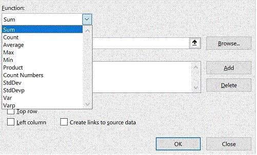
Multiple calculations can be made in a single formula using ________- a)Standard Formulas
- b)Array Formula
- c)Complex Formulas
- d)Smart Formula
Correct answer is option 'B'. Can you explain this answer?
Multiple calculations can be made in a single formula using ________
a)
Standard Formulas
b)
Array Formula
c)
Complex Formulas
d)
Smart Formula
|
|
Amar Singh answered |
Array Formulas are used in spreadsheets to perform multiple calculations in a single formula. They are a powerful tool that can save time and simplify complex calculations. Let's take a closer look at how they work.
What are Array Formulas?
An Array Formula is a formula that can perform calculations on a range of cells instead of a single cell. It can return multiple values or perform multiple calculations simultaneously. Array Formulas are enclosed in curly brackets {} and must be entered by pressing Ctrl+Shift+Enter instead of just Enter.
How do Array Formulas work?
Array Formulas use arrays, which are a collection of values, to perform calculations. The formula is applied to each value in the array, and the results are returned as an array of values. This allows multiple calculations to be performed at once.
Example
Let's say we have a list of numbers in cells A1 to A5, and we want to find the square of each number. Normally, we would have to enter the formula =A1^2 in cell B1, =A2^2 in cell B2, and so on. With an Array Formula, we can perform all the calculations in a single formula.
1. Select the range of cells where you want the results to be displayed, let's say B1 to B5.
2. Enter the formula =A1:A5^2 in cell B1.
3. Instead of pressing Enter, press Ctrl+Shift+Enter.
4. The formula will be surrounded by curly brackets {} to indicate that it is an Array Formula.
5. The result will be displayed in cells B1 to B5, showing the square of each number.
Advantages of Array Formulas
- Simplify complex calculations by performing multiple calculations in a single formula.
- Save time by avoiding the need to enter formulas in multiple cells.
- Perform calculations on a range of cells instead of a single cell.
Conclusion
Array Formulas are a powerful feature in spreadsheets that allow multiple calculations to be performed in a single formula. They can simplify complex calculations and save time by performing calculations on a range of cells. By understanding how to use Array Formulas, you can enhance your spreadsheet skills and perform calculations more efficiently.
By default Excel provides 3 worksheets. You need only two of them, how will you delete the third one?- a)Right click on Sheet Tab of third sheet and choose Delete from the context menu
- b)Click on Sheet 3 and from Edit menu choose Delete
- c)Both of above
- d)None of above
Correct answer is option 'A'. Can you explain this answer?
By default Excel provides 3 worksheets. You need only two of them, how will you delete the third one?
a)
Right click on Sheet Tab of third sheet and choose Delete from the context menu
b)
Click on Sheet 3 and from Edit menu choose Delete
c)
Both of above
d)
None of above
|
|
Utkarsh Joshi answered |
Right-click the tab and choose Delete from its shortcut menu in All version of excel.
In Microsoft Excel 2010 onwards Choose Home > Delete > Delete Sheet on the Ribbon, press Alt+HDS
Microsoft Excel 2007 and earlier Press ‘ALT’ + ‘E’, then the ‘L’ key.
In Microsoft Excel 2010 onwards Choose Home > Delete > Delete Sheet on the Ribbon, press Alt+HDS
Microsoft Excel 2007 and earlier Press ‘ALT’ + ‘E’, then the ‘L’ key.
Which of the following action removes a sheet from workbook?- a)Select the sheet, then choose Edit > Delete Sheet
- b)Select the sheet then choose Format > Sheet > Hide
- c)Both of above
- d)None of above
Correct answer is option 'A'. Can you explain this answer?
Which of the following action removes a sheet from workbook?
a)
Select the sheet, then choose Edit > Delete Sheet
b)
Select the sheet then choose Format > Sheet > Hide
c)
Both of above
d)
None of above
|
|
Parth Das answered |
Delete Sheet
b)Right-click the sheet tab, then choose Delete
c)Click the Home tab, then choose Delete Sheet
d)Press the Delete key on the keyboard
b)Right-click the sheet tab, then choose Delete
c)Click the Home tab, then choose Delete Sheet
d)Press the Delete key on the keyboard
Comments can be added to cells using ________- a)Home > Comments
- b)Insert > Comment
- c)Data > Comments
- d)Review > Comments
Correct answer is option 'D'. Can you explain this answer?
Comments can be added to cells using ________
a)
Home > Comments
b)
Insert > Comment
c)
Data > Comments
d)
Review > Comments
|
|
Utkarsh Joshi answered |
Comments can be added to cells using Review > Comment.
Paste Special allows some operation while you paste to new cell. Which of the following operation is valid?- a)Square
- b)Percentage
- c)Goal Seek
- d)Divide
Correct answer is option 'D'. Can you explain this answer?
Paste Special allows some operation while you paste to new cell. Which of the following operation is valid?
a)
Square
b)
Percentage
c)
Goal Seek
d)
Divide
|
|
Saikat Mehta answered |
Understanding Paste Special in Excel
Paste Special is a powerful feature in Excel that allows users to perform various operations while pasting data. It offers options beyond standard pasting, enabling manipulation of the copied data in different ways. Among the options presented, let's explore the valid operation.
Valid Operation: Divide
- When using Paste Special, one can divide the values of the copied cells by the values in the destination cells. This operation is particularly useful for adjusting datasets proportionally.
Explanation of Other Options
- Square: There is no direct option in Paste Special to square the values. The available mathematical operations include addition, subtraction, multiplication, and division, but squaring is not among them.
- Percentage: While you can calculate percentages in Excel, there is no Paste Special function specifically for directly converting values to percentages. You would typically need to format the cell after pasting.
- Goal Seek: This is a separate tool used for finding a specific value by adjusting other values in a formula. It does not relate to the Paste Special function.
Conclusion
In summary, among the options provided, only the "Divide" operation is valid within the Paste Special functionality. This feature enhances data management capabilities, allowing users to perform arithmetic operations conveniently. Mastering these tools is essential for effective data handling in Excel.
To remove the content of selected cells you must issue ______ command- a)Delete
- b)Clear Contents
- c)Clear All
- d)Clear Delete
Correct answer is option 'B'. Can you explain this answer?
To remove the content of selected cells you must issue ______ command
a)
Delete
b)
Clear Contents
c)
Clear All
d)
Clear Delete
|
|
Surbhi Patel answered |
Explanation:
To remove the content of selected cells in a spreadsheet, the correct command to use is "Clear Contents". This command is used to clear the data within the selected cells while keeping the formatting intact.
Here is a detailed explanation of the available options and why "Clear Contents" is the correct choice:
1. Delete:
The "Delete" command is used to permanently remove entire rows, columns, or cells from the spreadsheet. It not only removes the content but also deletes the cells themselves. This is not the desired action if the goal is to only remove the content while preserving the cell structure.
2. Clear All:
The "Clear All" command removes both the content and the formatting of the selected cells. It completely clears all the data and formatting, returning the cells to their default state. This is not the desired action if you want to keep the formatting intact.
3. Clear:
The "Clear" command is a general option that allows you to choose what elements to clear within the selected cells. It provides options to clear contents, formatting, hyperlinks, comments, and more. To remove the content while preserving the formatting, you need to specifically choose the "Clear Contents" option.
4. Clear Contents:
The "Clear Contents" command is designed to remove only the content within the selected cells, while leaving the formatting, formulas, and other cell properties intact. It is the correct command to use when you want to delete the data but keep the structure and appearance of the cells.
Therefore, the correct command to remove the content of selected cells is "Clear Contents" (option B). It allows you to delete the data while preserving the formatting and other cell properties.
Edit > Delete command- a)Deletes the content of a cell
- b)Deletes Formats of cell
- c)Deletes the comment of cell
- d)Deletes selected cells
Correct answer is option 'D'. Can you explain this answer?
Edit > Delete command
a)
Deletes the content of a cell
b)
Deletes Formats of cell
c)
Deletes the comment of cell
d)
Deletes selected cells
|
|
Mihir Menon answered |
Understanding the Delete Command
The Delete command in spreadsheet applications is a crucial feature that enables users to manage their data efficiently. Among the options provided, the correct answer is option 'D', which refers to deleting selected cells.
What Does Deleting Selected Cells Mean?
- Deleting selected cells removes the entire cell(s) and shifts the surrounding data to fill the gap.
- This action can be applied to one or multiple cells, allowing for flexible data management.
Analysis of Other Options
- a) Deletes the content of a cell:
- This option refers to clearing the data within a cell but does not remove the cell itself.
- b) Deletes Formats of cell:
- This action would reset the formatting of a cell (like font style, color, etc.) without affecting the actual data present.
- c) Deletes the comment of cell:
- This option pertains to removing any comments attached to a cell, which does not involve the cell's content or its structure.
Why Option D is Correct?
- Option 'D' is the most comprehensive choice because it signifies the removal of entire cells rather than just their content, formatting, or comments.
- This command is essential for organizing data, as it allows users to restructure their spreadsheets by eliminating unnecessary cells.
In conclusion, understanding the distinction between these options is vital for effective data management in spreadsheets, especially for students learning how to use these tools.
In EXCEL, you can sum a large range of data by simply selecting a tool button called ________.- a)AutoFill
- b)Auto correct
- c)Auto sum
- d)Auto format
Correct answer is option 'C'. Can you explain this answer?
In EXCEL, you can sum a large range of data by simply selecting a tool button called ________.
a)
AutoFill
b)
Auto correct
c)
Auto sum
d)
Auto format
|
|
Utkarsh Joshi answered |
AutoSum is a Microsoft Excel function that adds together a range of cells and displays the total in the cell below the selected range.
Which Chart can be created in Excel?- a)Area
- b)Line
- c)Pie
- d)All of the above
Correct answer is option 'D'. Can you explain this answer?
Which Chart can be created in Excel?
a)
Area
b)
Line
c)
Pie
d)
All of the above
|
|
Utkarsh Joshi answered |
Excel offers the following major chart types −
- Column Chart
- Line Chart
- Pie Chart
- Doughnut Chart
- Bar Chart
- Area Chart
- XY (Scatter) Chart
- Bubble Chart
- Stock Chart
- Surface Chart
- Radar Chart
- Combo Chart
The shortcut key Ctrl + R is used in Excel to- a)Right align the content of cell
- b)Remove the cell contents of selected cells
- c)Fill the selection with active cells to the right
- d)None of above
Correct answer is option 'C'. Can you explain this answer?
The shortcut key Ctrl + R is used in Excel to
a)
Right align the content of cell
b)
Remove the cell contents of selected cells
c)
Fill the selection with active cells to the right
d)
None of above
|
|
Utkarsh Joshi answered |
Ctrl+R fills the row cell to the right with the contents of the selected cell. To fill more than one cell, select the source cell and press Ctrl+Shift+Right arrow to select multiple cells. Then press Ctrl+R to fill them with the contents of the original cell.
The command Edit > Fill Across Worksheet is active only when- a)One sheet is selected
- b)When many sheets are selected
- c)When no sheet is selected
- d)None of above
Correct answer is option 'B'. Can you explain this answer?
The command Edit > Fill Across Worksheet is active only when
a)
One sheet is selected
b)
When many sheets are selected
c)
When no sheet is selected
d)
None of above
|
|
Kunal Ghosh answered |
The "Edit" command is a common command used in computer programs and applications to modify or change the content of a file, document, or text. It allows the user to make changes such as adding, deleting, or modifying text, images, formatting, and other elements. The specific functionality and options available within the Edit command can vary depending on the program or application being used.
Which menu option can be used to split windows into two?- a)Review > Window
- b)View > Window > Split
- c)Window > Split
- d)View > Split
Correct answer is option 'B'. Can you explain this answer?
Which menu option can be used to split windows into two?
a)
Review > Window
b)
View > Window > Split
c)
Window > Split
d)
View > Split
|
|
Utkarsh Joshi answered |
View > Window > Split option can be used to split windows into two.
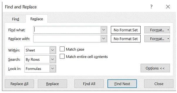
Which of the following is not true about Find and Replace in Excel- a)You can search for bold and replace with italics
- b)You can decide whether to look for the whole word or not
- c)You can search in formula too
- d)You can search by rows or columns or sheets
Correct answer is option 'A'. Can you explain this answer?
Which of the following is not true about Find and Replace in Excel
a)
You can search for bold and replace with italics
b)
You can decide whether to look for the whole word or not
c)
You can search in formula too
d)
You can search by rows or columns or sheets
|
|
Utkarsh Joshi answered |
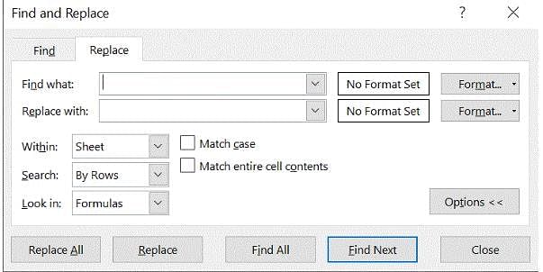
What is the shortcut key to replace a data with another in sheet?- a)Ctrl + R
- b)Ctrl + Shift + R
- c)Ctrl + H
- d)Ctrl + F
Correct answer is option 'C'. Can you explain this answer?
What is the shortcut key to replace a data with another in sheet?
a)
Ctrl + R
b)
Ctrl + Shift + R
c)
Ctrl + H
d)
Ctrl + F
|
|
Utkarsh Joshi answered |
Ctrl + H shortcut key is usedto replace a data with another in sheet.
While Finding and Replacing some data in Excel, which of the following statement is valid?- a)You can Find and Replace within the sheet or workbook
- b)Excel does not have option to match case for find
- c)Both are valid
- d)None are valid
Correct answer is option 'A'. Can you explain this answer?
While Finding and Replacing some data in Excel, which of the following statement is valid?
a)
You can Find and Replace within the sheet or workbook
b)
Excel does not have option to match case for find
c)
Both are valid
d)
None are valid
|
|
Utkarsh Joshi answered |
In Excel we can Find and Replace within the sheet or workbook.
How do you rearrange the data in ascending or descending order?- a)Data, Sort
- b)Data, Form
- c)Data, Table
- d)Data Subtotals
Correct answer is option 'A'. Can you explain this answer?
How do you rearrange the data in ascending or descending order?
a)
Data, Sort
b)
Data, Form
c)
Data, Table
d)
Data Subtotals
|
|
Utkarsh Joshi answered |
Sorting data in MS Excel rearranges the rows based on the contents of a particular column. We can also sort a table to put names in alphabetical order or ascending or descending order. Or, maybe we want to sort data by Amount from smallest to largest or largest to smallest.
How do you display current date and time in MS Excel?- a)Date ()
- b)Today ()
- c)Now ()
- d)Time ()
Correct answer is option 'C'. Can you explain this answer?
How do you display current date and time in MS Excel?
a)
Date ()
b)
Today ()
c)
Now ()
d)
Time ()
|
|
Utkarsh Joshi answered |
DATE - returns the serial date value for a date
TODAY - returns today's date
NOW - returns the current date and time
TIME - assemble a proper time.
TODAY - returns today's date
NOW - returns the current date and time
TIME - assemble a proper time.
Chapter doubts & questions for Excel Tips - How to become an Expert of MS Excel 2025 is part of Class 6 exam preparation. The chapters have been prepared according to the Class 6 exam syllabus. The Chapter doubts & questions, notes, tests & MCQs are made for Class 6 2025 Exam. Find important definitions, questions, notes, meanings, examples, exercises, MCQs and online tests here.
Chapter doubts & questions of Excel Tips - How to become an Expert of MS Excel in English & Hindi are available as part of Class 6 exam.
Download more important topics, notes, lectures and mock test series for Class 6 Exam by signing up for free.
How to become an Expert of MS Excel
92 videos|62 docs|15 tests
|
|
© EduRev
|
Education Revolution
|


|


Signup to see your scores
go up within 7 days!
Access 1000+ FREE Docs, Videos and Tests
Takes less than 10 seconds to signup